14. Introduction to GPU computing with CUDA and PyTorch#
How GPU computing works.
NVIDIA hardware and CUDA.
Host and Device parts of code.
Threads, blocks, warps, SIMT.
GPU memory management.
Code compilation and run.
Neural networks quick introduiction.
Jupyter hub access.
Pytorch exercises with neural networks.
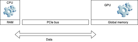
14.1. HOW GPU accelerated computing works#
Application runs essentially on a CPU
Some procedures can run on GPU
Data is sent back and forth between the devices over PCIe bus
CPU and GPU run cycles independently
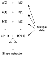
14.2. Type of compute tasks to run on GPU#
Single Instruction Multiple Data (SIMD) simulations can efficiently run across many light weight threads on GPU Stream Multiprocessors.
For example, vector sum:
14.3. GPU computing cons and pros#
Two types of programming environments: CUDA and OpenAcc (less performance efficient).
Pros:
computing power for Single Instruction Multiple Data tasks thanks to available many GPU threads.
Many applications are already developed and ported into CUDA: Matlab, Comsol, VASP, python wrappers (pycuda).
Good for neural network comuting since it is based on the tensor algebra.
Cons:
Not beneficial for non SIMD computing.
Nontrivial programming in CUDA.
Hardware - CUDA compatibility and dependency on Nvidia support. Relatively old GPU hardware is no longer supported by latest CUDA releases.
14.4. Host and Device parts of a code#
Data is initialized and may be computed on the CPU (host part)
CPU calls to allocate memory space for DATA on GPU (host part)
CPU sends data to the GPU (host part)
CPU invokes GPU part of the code, kernel, to execute (device part)
GPU executes its code (device part)
CPU receives data from GPU (host part)
Example: hello.cu, without data send/receive. The global is the device directive
#include<stdio.h>
#include<stdlib.h>

//Kernel definition (device part):
   __global__ void print_from_gpu(void) {
       printf("Hello World! from thread [%d,%d]From device\n", threadIdx.x,blockIdx.x);
}

//Host part:
int main(void) {
       printf("Hello World from host!\n");
    // Kernel invocation with 2 threads
       print_from_gpu<<<1,2>>>();
       cudaDeviceSynchronize();
       return 0;
}
Example: vector_add.cu code snipped with data send/receive:
// Device code
__global__ void VecAdd(float* A, float* B, float* C, int N)
{
    int i = blockDim.x * blockIdx.x + threadIdx.x;
    if (i < N)
        C[i] = A[i] + B[i];
}

// Host code
int main()
{
    int N = ...;
    size_t size = N * sizeof(float);

    // Allocate input vectors h_A and h_B in host memory
    float* h_A = (float*)malloc(size);
    float* h_B = (float*)malloc(size);

    // Initialize input vectors
    ...

    // Allocate vectors in device memory
    float* d_A;
    cudaMalloc(&d_A, size);
    float* d_B;
    cudaMalloc(&d_B, size);
    float* d_C;
    cudaMalloc(&d_C, size);

    // Copy vectors from host memory to device memory
    cudaMemcpy(d_A, h_A, size, cudaMemcpyHostToDevice);
    cudaMemcpy(d_B, h_B, size, cudaMemcpyHostToDevice);

    // Invoke kernel
    int threadsPerBlock = 256;
    int blocksPerGrid = (N + threadsPerBlock - 1) / threadsPerBlock;
    VecAdd<<<blocksPerGrid, threadsPerBlock>>>(d_A, d_B, d_C, N);

    // Copy result from device memory to host memory
    // h_C contains the result in host memory
    cudaMemcpy(h_C, d_C, size, cudaMemcpyDeviceToHost);

    // Free device memory
    cudaFree(d_A);
    cudaFree(d_B);
    cudaFree(d_C);

    // Free host memory
    ...
}
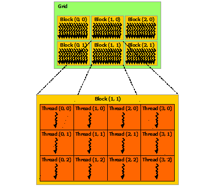
14.5. Threads, blocks, warps, and grid#
Single computing operation on GPU is done by a
thread.Threads are grouped into a
block.The number of threads in a block is defined by the code developer.
Each block performs the same operation on all its threads.
CUDA employs a Single Instruction Multiple Thread (SIMT) architecture to manage and execute threads in groups of 32 called
warps.Data for each thread may be different.
The blocks are scheduled and run independently of each other.
Blocks are organized into a one-dimensional, two-dimensional, or three-dimensional
gridof thread blocks.
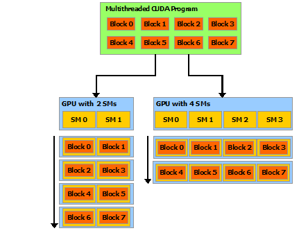
14.6. Blocks on Streaming Multiprocessors (SM)#
A GPU with more multiprocessors will automatically execute the program in less time than a GPU with fewer multiprocessors.
14.7. Thread indexing#
Each thread in the grid is uniquely identified by its index,
ix.There is also the thread index within a block,
threadIdx.x.Each block within the grid can be identified by its own index,
blockIdx.xThe relationship between the indexes:
int i = blockIdx.x * blockDim.x + threadIdx.x;
where blockDim.x is the size of the block.
For convenience of computing multi-dimensional data, the indexes can be defined as one-dimensional, two-dimensional, or three-dimensional:
int ix = blockIdx.x * blockDim.x + threadIdx.x;
int iy = blockIdx.y * blockDim.y + threadIdx.y;
int iz = blockIdx.z * blockDim.z + threadIdx.z;
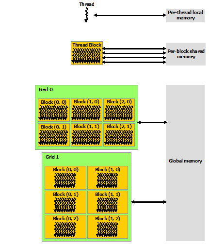
14.8. Memory Hierarchy#
CUDA threads may access data from multiple memory spaces during their execution.
Each thread has private
local memory.Each thread block has
shared memoryvisible to all threads of the block and with the same lifetime as the block.All threads have access to the same
global memory.Data from the host arrives into and departs from the
global memory. Theglobal memoryis much slower than the other two.There are also two additional read-only memory spaces accessible by all threads: the constant and texture memory spaces.
14.9. The main challenge in CUDA computing is memory management#
Data from the host arrives into the
global memory, the slowest type of memory on th GPU.One should avoid using the
global memoryfor thread computing. Copy data into theshared memory, compute, then copy results back into theglobal memory.Another challenge often happens due to noncalescent data alignment in
global memory. Data is read inwarpsof size 32. For unstructured data, it may take multiple warp cycles to load the data into theshared memory.
14.10. Example: matrix multiplication#
[C] = [A] x [B]
In terms of matrix elements:
\(c_{ij} = \Sigma_{k} a_{ik} b_{kj}\)
Review and comparison:
Computing on the
global memory.Computing on the
shared memory.
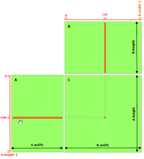
14.11. Thread computing on the global memory.#
// Matrices are stored in row-major order:
// M(row, col) = *(M.elements + row * M.width + col)
typedef struct {
    int width;
    int height;
    float* elements;
} Matrix;

// Thread block size
#define BLOCK_SIZE 16

// Forward declaration of the matrix multiplication kernel
__global__ void MatMulKernel(const Matrix, const Matrix, Matrix);

// Matrix multiplication - Host code
// Matrix dimensions are assumed to be multiples of BLOCK_SIZE
void MatMul(const Matrix A, const Matrix B, Matrix C)
{

    // Load A and B to device memory
    Matrix d_A;
    d_A.width = A.width; d_A.height = A.height;
    size_t size = A.width * A.height * sizeof(float);
    cudaMalloc(&d_A.elements, size);
    cudaMemcpy(d_A.elements, A.elements, size, cudaMemcpyHostToDevice);
    Matrix d_B;
    d_B.width = B.width; d_B.height = B.height;
    size = B.width * B.height * sizeof(float);
    cudaMalloc(&d_B.elements, size);
    cudaMemcpy(d_B.elements, B.elements, size, cudaMemcpyHostToDevice);

    // Allocate C in device memory
    Matrix d_C;
    d_C.width = C.width; d_C.height = C.height;
    size = C.width * C.height * sizeof(float);
    cudaMalloc(&d_C.elements, size);

    // Invoke kernel
    dim3 dimBlock(BLOCK_SIZE, BLOCK_SIZE);
    dim3 dimGrid(B.width / dimBlock.x, A.height / dimBlock.y);

    MatMulKernel<<<dimGrid, dimBlock>>>(d_A, d_B, d_C);

    // Read C from device memory
    cudaMemcpy(C.elements, d_C.elements, size, cudaMemcpyDeviceToHost);

    // Free device memory
    cudaFree(d_A.elements);
    cudaFree(d_B.elements);
    cudaFree(d_C.elements);
}
// Matrix multiplication kernel called by MatMul()
__global__ void MatMulKernel(Matrix A, Matrix B, Matrix C)
{
    // Each thread computes one element of C
    // by accumulating results into Cvalue
    float Cvalue = 0;
    int row = blockIdx.y * blockDim.y + threadIdx.y;
    int col = blockIdx.x * blockDim.x + threadIdx.x;
    for (int e = 0; e < A.width; ++e)
      Cvalue += A.elements[row * A.width + e] * B.elements[e * B.width + col];
      C.elements[row * C.width + col] = Cvalue;
}
14.12. Computing with the shared memory#
Threads in their own blocks compute the product on the submatrices, then copy the result into the global memory.
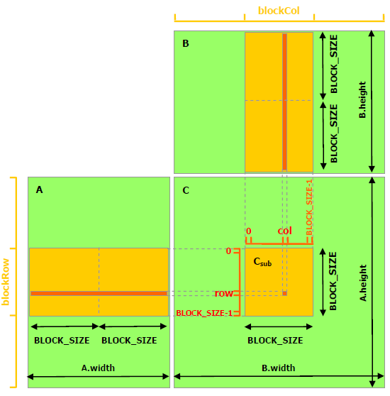
// Matrices are stored in row-major order:
// M(row, col) = *(M.elements + row * M.stride + col)
typedef struct {
    int width;
    int height;
    int stride;
    float* elements;
} Matrix;

// Get a matrix element
__device__ float GetElement(const Matrix A, int row, int col)
{
    return A.elements[row * A.stride + col];
}

// Set a matrix element
__device__ void SetElement(Matrix A, int row, int col,
                           float value)
{
    A.elements[row * A.stride + col] = value;
}

// Get the BLOCK_SIZExBLOCK_SIZE sub-matrix Asub of A that is
// located col sub-matrices to the right and row sub-matrices down
// from the upper-left corner of A
 __device__ Matrix GetSubMatrix(Matrix A, int row, int col)
{
    Matrix Asub;
    Asub.width    = BLOCK_SIZE;
    Asub.height   = BLOCK_SIZE;
    Asub.stride   = A.stride;
    Asub.elements = &A.elements[A.stride * BLOCK_SIZE * row
                                         + BLOCK_SIZE * col];
    return Asub;
}

// Thread block size
#define BLOCK_SIZE 16

// Forward declaration of the matrix multiplication kernel
__global__ void MatMulKernel(const Matrix, const Matrix, Matrix);

// Matrix multiplication - Host code
// Matrix dimensions are assumed to be multiples of BLOCK_SIZE
void MatMul(const Matrix A, const Matrix B, Matrix C)
{
    // Load A and B to device memory
    Matrix d_A;
    d_A.width = d_A.stride = A.width; d_A.height = A.height;
    size_t size = A.width * A.height * sizeof(float);
    cudaMalloc(&d_A.elements, size);
    cudaMemcpy(d_A.elements, A.elements, size, cudaMemcpyHostToDevice);
    Matrix d_B;
    d_B.width = d_B.stride = B.width; d_B.height = B.height;
    size = B.width * B.height * sizeof(float);
    cudaMalloc(&d_B.elements, size);
    cudaMemcpy(d_B.elements, B.elements, size, cudaMemcpyHostToDevice);

    // Allocate C in device memory
    Matrix d_C;
    d_C.width = d_C.stride = C.width; d_C.height = C.height;
    size = C.width * C.height * sizeof(float);
    cudaMalloc(&d_C.elements, size);

    // Invoke kernel
    dim3 dimBlock(BLOCK_SIZE, BLOCK_SIZE);
    dim3 dimGrid(B.width / dimBlock.x, A.height / dimBlock.y);
    MatMulKernel<<<dimGrid, dimBlock>>>(d_A, d_B, d_C);

    // Read C from device memory
    cudaMemcpy(C.elements, d_C.elements, size, cudaMemcpyDeviceToHost);

    // Free device memory
    cudaFree(d_A.elements);
    cudaFree(d_B.elements);
    cudaFree(d_C.elements);
}

// Matrix multiplication kernel called by MatMul()
 __global__ void MatMulKernel(Matrix A, Matrix B, Matrix C)
{
    // Block row and column
    int blockRow = blockIdx.y;
    int blockCol = blockIdx.x;

    // Each thread block computes one sub-matrix Csub of C
    Matrix Csub = GetSubMatrix(C, blockRow, blockCol);

    // Each thread computes one element of Csub
    // by accumulating results into Cvalue
    float Cvalue = 0;

    // Thread row and column within Csub
    int row = threadIdx.y;
    int col = threadIdx.x;

    // Loop over all the sub-matrices of A and B that are
    // required to compute Csub
    // Multiply each pair of sub-matrices together
    // and accumulate the results
    for (int m = 0; m < (A.width / BLOCK_SIZE); ++m) {

        // Get sub-matrix Asub of A
        Matrix Asub = GetSubMatrix(A, blockRow, m);

        // Get sub-matrix Bsub of B
        Matrix Bsub = GetSubMatrix(B, m, blockCol);

        // Shared memory used to store Asub and Bsub respectively
        __shared__ float As[BLOCK_SIZE][BLOCK_SIZE];
        __shared__ float Bs[BLOCK_SIZE][BLOCK_SIZE];

        // Load Asub and Bsub from device memory to shared memory
        // Each thread loads one element of each sub-matrix
        As[row][col] = GetElement(Asub, row, col);
        Bs[row][col] = GetElement(Bsub, row, col);

        // Synchronize to make sure the sub-matrices are loaded
        // before starting the computation
        __syncthreads();
        // Multiply Asub and Bsub together
        for (int e = 0; e < BLOCK_SIZE; ++e)
            Cvalue += As[row][e] * Bs[e][col];

        // Synchronize to make sure that the preceding
        // computation is done before loading two new
        // sub-matrices of A and B in the next iteration
        __syncthreads();
    }

    // Write Csub to device memory
    // Each thread writes one element
    SetElement(Csub, row, col, Cvalue);
}
14.13. Access a GPU VM (Exercise)#
SSH to one of the VMs, which have Nvidia T4, CUDA installed and PyTorch configured. For the user name and password, use your Engineering account.
GPU VM 1:
ssh -p 60097 -L 8000:localhost:8000 user_name@172.16.26.101
GPU VM 2:
ssh -p 60100 -L 8000:localhost:8000 user_name@172.16.26.102
GPU VM 3:
ssh -p 60094 -L 8000:localhost:8000 user_name@172.16.26.103
14.14. Setup the environment for CUDA nvcc code compilation (Exercise)#
CUDA 13.2 Toolkit is already installed on the dedicated virtual desktops.
CUDA compiler,
nvccis part of the ToolkitNeed to set the PATH environment variable to access the Nvidia toolkit: in your
.bashrcadd the two lines:
export PATH=/usr/local/cuda-13.2/bin${PATH:+:${PATH}}
export LD_LIBRARY_PATH=/usr/local/cuda-13.2/lib64${LD_LIBRARY_PATH:+:${LD_LIBRARY_PATH}}
Run
bash source .bashrc
Check if the nvidia driver is loaded and the operating system can communicate with the GPU:
nvidia-smi
Create directory CUDA:
mkdir CUDA
Copy deviceQuery.cpp source code into directory CUDA, and compile it:
cd CUDA
nvcc -o deviceQuery deviceQuery.cpp -I /usr/local/cuda-samples/Common
Run the executable to see the prameters of the GPU card on your desktop:
./deviceQuery
14.15. Compile and run hello.cu (Exercise)#
in directory CUDA, download a tar ball with cuda source codes, and extract the files:
wget http://linuxcourse.rutgers.edu/2024/html/lessons/HPC_3/GPU.tgz
tar -zxvf GPU.tgz
Compile and run hello.cu:
nvcc -o hello hello.cu
./hello
Edit file hello.cu, and change the number of blocks to 4 and threads per block to 8 in the line that starts the device code:
print_from_gpu<<<4,8>>>();
Recompile and run the code:
nvcc -o hello hello.cu
./hello
See how the output from the blocks and the threads changes.
14.16. Compile and run the matrix multiplication codes (Exercise)#
A routine that computes the wallclock time for the device function has been added in the both matrix multiplication codes discussed above.
Compile and run the code with global memory computation:
nvcc -o matrix_mult  matrix_mult.cu
./matrix_mult
Compile and run the code with shard memory computation:
nvcc -o matrix_mult_shared matrix_mult_shared.cu
./matrix_mult_shared
Compare the printed out wall clock times of the device part. Notice that matrix_mult_shared runs about 2.6 times faster than matrix_mult.
14.17. CUDA enabled programming environments#
For example: Matlab and Python
CUDA support in Python comes in PyTorch, TensorFlow, pybind11, etc.
14.18. Perceptron#
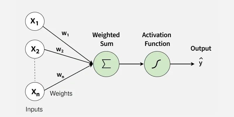
Neural network model: \(\hat{y} = f(\Sigma w_i\;x_i + b)\)
Input parameters: \(X = (x_1, x_2, ..., x_n)\)
Weights: \(W = (w_1, w_2, ..., w_n)\)
Bias: \(b\)
Nonlinear activation function: \(f\)
True data: \(y\)
Modeled result: \(\hat{y}\)
Loss or error \(\delta y = y - \hat{y}\)
Iterative training update of the weights: \(w_i = w_i + \eta \; (y - \hat{y})\). Also called back propagation.
Iterative training update of the bias: \(b = b + \eta \; (y - \hat{y})\). There are different algorithms that can be used for computing \(\eta\).
The training finalizes the model with \((w_1, w_2, ..., w_n)\) and \(b\).
After training, the model can be used for predicting the final outome for new input parameters.
14.19. Neural networks#
In practical cases, the perceptrons are combined into neural networks.
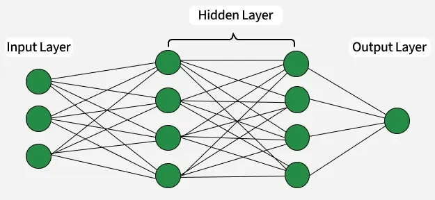
Python based PyTorch is a suit of methods for computing with neural networks.
14.20. Jupyter hub access#
Navigate your browser to:
http://localhost:8000
Login to the Jupyter hub with the same Engineering account.
14.21. Exercises with Pytorch#
In your home directory of the GPU VM, create directory Python and download cuda_Pytorch_sonar.ipynb into the directory:
mkdir Python
cd Python
wget --no-check-certificate https://linuxcourse.rutgers.edu/Files/cuda_Pytorch_sonar.ipynb
Navigate your Juputer lab to the file and load it in the cells.
Alternatively, you can copy/paste the code below into a Jupyter cell.
We utilize the Sonar, Mines vs. Rocks dataset downloaded from University of Chicago.
It is directly downloadable into Pandas dataframe.
By using StratifiedKFold module, we split the dataset into 80% training and 20% testing.
We utilize two models:
with 1 hidden layer
with 3 hidden layers
Apply the Mean Square Errors and Adam optimizer for back propagation.
14.22. The “Sonar, Mines vs Rocks” code on GPU.#
%%script false --no-raise-error

# Import Pytorch
import torch

# If available, assign the device to GPU and print the GPU type
if torch.cuda.is_available():
    device = torch.device("cuda")
    print(f"GPU Device: {torch.cuda.get_device_name(0)}")
else:
    device = torch.device("cpu")

# Import neural networks and optimizers from the Torch:
import torch.nn as nn
import torch.optim as optim

# Import the modules for data preprocessing:
import numpy as np
import pandas as pd
from sklearn.model_selection import StratifiedKFold, train_test_split

# Import Sonar dataset module with experimental sonar measurements.
from ucimlrepo import fetch_ucirepo

connectionist_bench_sonar_mines_vs_rocks = fetch_ucirepo(id=151)

# Pull the sonar data into pandas dataframes
X = connectionist_bench_sonar_mines_vs_rocks.data.features
y = connectionist_bench_sonar_mines_vs_rocks.data.targets

# metadata
print(connectionist_bench_sonar_mines_vs_rocks.metadata)

# variable information
print(connectionist_bench_sonar_mines_vs_rocks.variables)

# Digitize the output values:
y = y.replace('R',float(1))
y = y.replace('M',float(0))

# Check the data type of X and y:
type(X)
type(y)

# Preprocess pandas dataframes into numpy arrays:
X = X.values
y = y['class'].values
y = y.astype(np.float32)

# Again, check the data type of X and y:
type(X)
type(y)

# Import the numpy arrays into the torch tensors
X = torch.FloatTensor(X)
y = torch.FloatTensor(y)

# Again, check the data type of X and y:
type(X)
type(y)

# Define a one layer neural model. It works OK here.
class sonar_neural_1(nn.Module):
    def __init__(self,input_size,hidden_size1,output_size):
        super().__init__()
        self.layer1 = nn.Linear(input_size, hidden_size1)
        self.act1 = nn.ReLU()
        self.output = nn.Linear(hidden_size1, output_size)

    def forward(self, x):
        x = self.layer1(x)
        x = self.act1(x)
        x = self.output(x)
        return x

# Define a 3 layer neural model. It works better here than the above.
class sonar_neural_3(nn.Module):
    def __init__(self,input_size,hidden_size,output_size):
        super().__init__()
        self.layer1 = nn.Linear(input_size, hidden_size)
        self.act1 = nn.ReLU()
        self.layer2 = nn.Linear(hidden_size, hidden_size)
        self.act2 = nn.ReLU()
        self.layer3 = nn.Linear(hidden_size, hidden_size)
        self.act3 = nn.ReLU()
        self.output = nn.Linear(hidden_size, 1)

    def forward(self, x):
        x = self.act1(self.layer1(x))
        x = self.act2(self.layer2(x))
        x = self.act3(self.layer3(x))
        x = self.output(x)
        return x

# k-fold data splitter. Split the X and y into the training and testing subsets: 80% and 20%, accordingly.
kfold = StratifiedKFold(n_splits=5, shuffle=True)

for train_index, test_index in kfold.split(X, y):
    X_train, X_test = X[train_index], X[test_index]
    y_train, y_test = y[train_index], y[test_index]

# Load the training data onto the GPU device
X_train = X_train.to(device)
y_train = y_train.to(device)

# Choose one of the two models defined above
model = sonar_neural_1(input_size = 60, hidden_size1=120, output_size= 1).to(device)
#model = sonar_neural_3(input_size = 60, hidden_size=30, output_size= 1).to(device)

# Set the criterion function that drives the weight updates
criterion = nn.MSELoss()  # Mean Square Errors

# set the optimizer a mathematical algorithm used to minimize the error (loss)
optimizer=   optim.Adam(model.parameters(),lr = 0.0001)

# Increases the tensor's dimensionality by one without changing its underlying data
y_train = y_train.unsqueeze(1)
y_test = y_test.unsqueeze(1)

# Proceed with iterative training
losses = []
num_epochs = 3000
for epoch in range(num_epochs):
  #Forward pass
  y_pred = model(X_train)
  loss = criterion(y_pred,y_train)

  #Backward Pass
  optimizer.zero_grad()
  loss.backward()
  optimizer.step()

  if epoch % 100 == 0:
    print(f'Epoch [{epoch}/100], Loss: {loss.item(): .4f}')
  losses.append(loss.item())

# Plot the loss value vs iterations
import matplotlib.pyplot as plt
plt.plot(range(num_epochs),losses)
plt.xlabel('Iteration')
plt.ylabel('Loss')
plt.title('Loss over itrations')
plt.show()

# The backtest on the 20% of the data:
with torch.no_grad():
  y_test_pred = model(X_test.to(device)).to(device)
  test_loss = criterion(y_test_pred,y_test.to(device))
  print(f'Test Loss: {test_loss.item():.4f}')

# The accuracy of the model
mae = torch.abs(y_test_pred - y_test.to(device)).mean()
print('Mean Absolute Error:',mae.item())
References: